main functions¶

The core functions of the tomography package.

tomography_tutorial.functions.calculate_covariance_matrix(img_stack, outname, kernelsize=10, overwrite=False)[source]¶

compute the covariance matrix. If the target file already exists and overwrite=False this function acts as a simple file reader.

Parameters:	img_stack (numpy.ndarray) – the normalized SLC image stack outname (str) – the name of the file to be written kernelsize (int) – the boxcar smoothing dimension overwrite (bool) – overwrite an existing file? Otherwise it is read from file and returned
Returns:	the covariance matrix
Return type:	numpy.ndarray

tomography_tutorial.functions.capon_beam_forming_inversion(covmatrix, kz_array, outname, height=70, overwrite=False)[source]¶

perform the capon beam forming inversion to create the final tomographic result. If the target file already exists and overwrite=False this function acts as a simple file reader.

Parameters:	covmatrix (numpy.ndarray) – the covariance matrix kz_array (numpy.ndarray) – the wave number stack outname (str) – the name of the file to be written height (int) – the maximum inversion height overwrite (bool) – overwrite an existing file? Otherwise it is read from file and returned
Returns:	the tomographic array
Return type:	numpy.ndarray

tomography_tutorial.functions.read_data(input, outname, overwrite=False)[source]¶

read the raw input data into a numpy array and write the results

Parameters:	input (str or list) – a single image file name or a list of multiple files outname (str) – the name of the file to be written. overwrite (bool) – overwrite an existing file? Otherwise it is read from file and returned
Returns:	an array in 2D (one file) or 3D (multiple files)
Return type:	numpy.ndarray

tomography_tutorial.functions.start(notebook)[source]¶

Create a custom copy of the jupyter notebook with a name defined buy the user and start it. The notebook is only copied from the package if it does not yet exist. Jupyter notebook files have the extension ‘.ipynb’. If the defined notebook does not contain this extension it is appended automatically.

Parameters:	directory (str) – the name of the custom notebook

tomography_tutorial.functions.topo_phase_removal(img_stack, dem_stack, outname, overwrite=False)[source]¶

Removal of Topographical Phase. If the target file already exists and overwrite=False this function acts as a simple file reader.

Parameters:	img_stack (numpy.ndarray) – the SLC image stack dem_stack (numpy.ndarray) – the image stack containing flat earth and topographic phase outname (str) – the name of the file to be written overwrite (bool) – overwrite an existing file? Otherwise it is read from file and returned
Returns:	the normalized SLC stack
Return type:	numpy.ndarray

ancillary functions¶

Additional general functions for the tomography package.

tomography_tutorial.ancillary.cbfi(slice, nTrack, height)[source]¶

computation of capon beam forming inversion for a single pixel. This function is used internally by the core function capon_beam_forming_inversion().

Parameters:	slice (numpy.ndarray) – an array containing the covariance matrix and wave number for a single pixel nTrack (int) – the number of original SLC files height (int) – the maximum inversion height
Returns:	the tomographic result for one pixel
Return type:	numpy.ndarray

tomography_tutorial.ancillary.geocode(data, lut_rg_name, lut_az_name, outname=None, range_min=0, range_max=None, azimuth_min=0, azimuth_max=None)[source]¶

Geocode a radar image using lookup tables. The LUTs are expected to be georeferenced and contain range and azimuth radar coordinates for a specific image data set which is linked to these LUTs. If parameter data is a subset of this data set, the pixel coordinates of this subset need to be defined.

Parameters:

data (numpy.ndarray) – the image data in radar coordinates
lut_rg_name (str) – the name of the range coordinates lookup table file
lut_az_name (str) – the name of the azimuth coordinates lookup table file
outname (str or None) – the name of the file to write; if None, the geocoded array is returned and no file is written. See function geowrite() for details on how the file is written.
range_min (int) – the minimum range coordinate
range_max (int) – the maximum range coordinate
azimuth_min (int) – the minimum azimuth coordinate
azimuth_max (int) – the maximum azimuth coordinate

Example

>>> from osgeo import gdal
>>> from tomography_tutorial.ancillary import geocode
>>> image_name = 'path/to/somedata/image.tif'
>>> lut_rg_name = 'path/to/somedata/lut_rg.tif'
>>> lut_az_name = 'path/to/somedata/lut_az.tif'
>>> outname = 'path/to/somedata/image_sub_geo.tif'
>>> image_ras = gdal.Open(image_name)
>>> image_mat = image_ras.ReadAsArray()
>>> image_ras = None
>>> image_mat_sub = image_mat[0:100, 200:400]
>>> geocode(image_mat_sub, outname, lut_rg_name, lut_az_name, range_min=200, range_max=400, azimuth_min=0, azimuth_max=100)

tomography_tutorial.ancillary.geowrite(data, outname, reference, indices, nodata=-99)[source]¶

write an array to a file using an already geocoded file as reference. The output format is either GeoTiff (for 2D arrays) or ENVI (for 3D arrays).

Parameters:

data (numpy.ndarray) – the array to write to the file; must be either 2D or 3D
outname (str) – the file name
reference (gdal.Dataset) – the geocoded reference dataset
indices (tuple of slices) – the slices which define the subset of data in reference, i.e. where is the data located within the reference pixel dimensions; see lut_crop()
nodata (int) – the nodata value to write to the file

tomography_tutorial.ancillary.listfiles(path, pattern)[source]¶

list files in a directory whose names match a regular expression

Parameters:	path (str) – the directory to be searched pattern (str) – the regular expression search pattern
Returns:	a list of absolute file names
Return type:	list

Example

>>> listfiles('/path/to/somedata', 'file[0-9].tif')
['/path/to/somedata/file1.tif', '/path/to/somedata/file2.tif', '/path/to/somedata/file3.tif']

tomography_tutorial.ancillary.lut_crop(lut_rg, lut_az, range_min=0, range_max=None, azimuth_min=0, azimuth_max=None)[source]¶

compute indices for subsetting the range and azimuth lookup tables (LUTs). The returned slices describe the minimum LUT subset, which contains all radar coordinates within the range-azimuth subset.

Parameters:	lut_rg (numpy.ndarray) – the lookup table for range direction lut_az (numpy.ndarray) – the lookup table for azimuth direction range_min (int) – first range pixel range_max (int) – last range pixel azimuth_min (int) – first azimuth pixel azimuth_max (int) – last azimuth pixel
Returns:	the pixel indices for subsetting: (ymin:ymax, xmin:xmax)
Return type:	tuple of slices

tomography_tutorial.ancillary.normalize(slice)[source]¶

normalize a 1D array by its minimum and maximum values:

$y = \frac{x-min(x)}{max(x)-min(x)}$

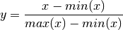
Parameters:	slice (numpy.ndarray) – the 1d input array to be normalized
Returns:	the normalized array
Return type:	numpy.ndarray

plotting¶

Plotting utilities for the Jupyter notebook.

class tomography_tutorial.plotting.DataViewer(slc_list, phase_list, kz_list, slc_stack, phase_stack, kz_stack)[source]¶

functionality for displaying the input data (SLC, topographic phase and wave number)

Parameters:

slc_list (list of str) – the names of the SLC input files
phase_list (list of str) – the names of the topographic phase input files
kz_list (list of str) – the names of the Kappa-Zeta wave number input files
slc_stack (numpy.ndarray) – the SLC images
phase_stack (numpy.ndarray) – the topographic phase images
kz_stack (numpy.ndarray) – the wave number images

class tomography_tutorial.plotting.GeoViewer(filename, cmap='jet', band_indices=None)[source]¶

plotting utility for displaying a geocoded image stack file.

On moving the slider, the band at the slider position is read from the file and displayed.

Parameters:

filename (str) – the name of the file to display
cmap (str) – the color map for displaying the image. See matplotlib.pyplot.imshow().
band_indices (list) – a list of indices for renaming the individual bands in filename such that one can scroll trough the range of inversion heights, e.g. -70:70, instead of the raw band indices, e.g. 1:140. The number of unique elements must of same length as the number of bands in filename.

class tomography_tutorial.plotting.Tomographyplot(capon_bf_abs, caponnorm)[source]¶

functionality for creating the main tomography_tutorial analysis plot

Parameters:	capon_bf_abs (numpy.ndarray) – the absolute result of the capon beam forming inversion caponnorm (numpy.ndarray) – the normalized version of capon_bf_abs; see function `normalize()`.